Manipulation of the data dictionary

What you’ll learn: Learn to quickly manipulate the subjects connectivity dictionary, selecting sub-sets of connectivity matrices regarding behavioral group or variables.

Author: Dhaif BEKHA

Retrieve the example dataset

In this example, we will work directly on a pre-computed dictionary, that contain two set of connectivity matrices, from two different groups. The first group, called controls is a set of connectivity matrices from healthy seven years old children, and the second group called patients, is a set of connectivity matrices from seven years old children who have suffered a stroke. You can download the dictionary use in this example here. You will also need, the data table containing a set of continuous or categorical behavioral variable regarding all the subjects in the dictionary. You can download the table here. When downloaded, all the files must be stored in your home directory.

Modules import

from conpagnon.data_handling import dictionary_operations, atlas, data_management
from conpagnon.utils.folders_and_files_management import load_object
import pandas as pd
from pathlib import Path
import os
import seaborn as sns
import matplotlib.pyplot as plt

Out:

/home/dhaif/anaconda3/envs/conpagnon/lib/python3.7/site-packages/sklearn/externals/joblib/__init__.py:15: DeprecationWarning: sklearn.externals.joblib is deprecated in 0.21 and will be removed in 0.23. Please import this functionality directly from joblib, which can be installed with: pip install joblib. If this warning is raised when loading pickled models, you may need to re-serialize those models with scikit-learn 0.21+.
  warnings.warn(msg, category=DeprecationWarning)

Load the data

We will first load the subjects connectivity dictionary, storing for each groups and subject, the connectivity matrices for different connectivity metric. We will also the corresponding data table.

# Fetch the path of the home directory
home_directory = str(Path.home())

# Load the dictionary containing the connectivity matrices
subjects_connectivity_matrices = load_object(
    full_path_to_object=os.path.join(home_directory, 'raw_subjects_connectivity_matrices.pkl'))

# load the data table
data_table = pd.read_excel(os.path.join(home_directory, 'data_table.xlsx'))
print(data_table.to_markdown())

# For convenience, we shift the index
# of the dataframe to the subjects
# identifiers column
data_table = data_table.set_index(['subjects'])

Out:

|    | subjects       | Group   | Sex   | Lesion   |      score |
|---:|:---------------|:--------|:------|:---------|-----------:|
|  0 | sub04_rc110343 | P       | M     | G        |   1.00484  |
|  1 | sub06_ml110125 | P       | M     | G        |   3.83867  |
|  2 | sub07_lc110496 | P       | M     | G        |  -0.907201 |
|  3 | sub08_jl110342 | P       | M     | G        |  -4.26892  |
|  4 | sub10_dl120547 | P       | M     | G        |  -0.957913 |
|  5 | sub12_ab110489 | P       | F     | G        |   3.21885  |
|  6 | sub13_vl110480 | P       | M     | G        |  -0.331407 |
|  7 | sub14_rs120006 | P       | M     | G        |  -1.05699  |
|  8 | sub17_eb120007 | P       | F     | G        |   2.88928  |
|  9 | sub20_hd120032 | P       | F     | D        |  -5.33207  |
| 10 | sub21_yg120001 | P       | M     | D        |  -1.56495  |
| 11 | sub23_lf120459 | P       | M     | D        |   3.80515  |
| 12 | sub24_ed110159 | P       | M     | D        | -10.4086   |
| 13 | sub25_ec110149 | P       | F     | D        |   1.78148  |
| 14 | sub26_as110192 | P       | M     | D        |  -3.93445  |
| 15 | sub30_zp130008 | P       | F     | G        |   1.42485  |
| 16 | sub32_mp130025 | P       | F     | G        |  -1.2626   |
| 17 | sub34_jc130100 | P       | M     | G        |   1.37514  |
| 18 | sub35_gc130101 | P       | M     | G        |   3.66906  |
| 19 | sub37_la130266 | P       | F     | D        |   3.77187  |
| 20 | sub38_mv130274 | P       | M     | D        |   2.17901  |
| 21 | sub39_ya130305 | P       | F     | G        |   1.08922  |
| 22 | sub41_sa130332 | P       | F     | D        |   1.80184  |
| 23 | sub43_mc130373 | P       | F     | G        |   2.01819  |
| 24 | sub44_av130474 | P       | F     | G        |  -3.84236  |
| 25 | sub01_nc110193 | C       | F     | nan      | nan        |
| 26 | sub02_ib110200 | C       | M     | nan      | nan        |
| 27 | sub03_ct110201 | C       | F     | nan      | nan        |
| 28 | sub04_eb110217 | C       | F     | nan      | nan        |
| 29 | sub05_gk110258 | C       | M     | nan      | nan        |
| 30 | sub06_al110271 | C       | M     | nan      | nan        |
| 31 | sub08_cd090095 | C       | F     | nan      | nan        |
| 32 | sub09_sl100362 | C       | M     | nan      | nan        |
| 33 | sub10_ag110427 | C       | M     | nan      | nan        |
| 34 | sub11_nn110428 | C       | F     | nan      | nan        |
| 35 | sub12_at110408 | C       | M     | nan      | nan        |
| 36 | sub14_rp120164 | C       | M     | nan      | nan        |
| 37 | sub16_cg120322 | C       | F     | nan      | nan        |
| 38 | sub17_cm120095 | C       | M     | nan      | nan        |
| 39 | sub18_cb130208 | C       | F     | nan      | nan        |
| 40 | sub19_cd120206 | C       | M     | nan      | nan        |
| 41 | sub20_mp120048 | C       | M     | nan      | nan        |
| 42 | sub21_sb120208 | C       | F     | nan      | nan        |
| 43 | sub22_ln120402 | C       | M     | nan      | nan        |
| 44 | sub23_kf130380 | C       | F     | nan      | nan        |
| 45 | sub24_ls130404 | C       | F     | nan      | nan        |
| 46 | sub25_sv120315 | C       | F     | nan      | nan        |
| 47 | sub26_ep120255 | C       | M     | nan      | nan        |
| 48 | sub27_ea130507 | C       | F     | nan      | nan        |
| 49 | sub28_ml130538 | C       | F     | nan      | nan        |
| 50 | sub29_hd130539 | C       | F     | nan      | nan        |

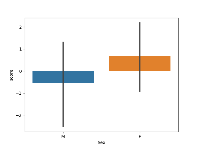
This data table have a very common structure with a mix of categorical and continous variable. Let’s barplot the score for the group of female and male in the patients population:

sns.barplot(x='Sex', y='score', data=data_table)
plt.show()

Out:

/media/dhaif/Samsung_T5/Work/Programs/ConPagnon/examples/05_utilities/plot_selection_of_data.py:74: UserWarning: Matplotlib is currently using agg, which is a non-GUI backend, so cannot show the figure.
  plt.show()

Selecting a subset of data

It’s common to extract and compute the connectivity matrices on your whole cohort of data, and entering them in one or multiple statistical analysis. In practice, you may want only selecting a sub-set of your connectivity matrices. For example, you might want to select inside the patients group, the left lesioned subject and male only. For convenience, and avoiding a fastidious manual extraction inside the subjects connectivity matrices dictionary, we create a special function dedicated to this task. The main inputs are the connectivity dictionary of your population and the corresponding table.

# Select the male, and left lesioned
# patients.
# Select a subset of patients
# Compute the connectivity matrices dictionary with factor as keys.
group_by_factor_subjects_connectivity, population_df_by_factor, factor_keys, = \
    dictionary_operations.groupby_factor_connectivity_matrices(
        population_data_file=os.path.join(home_directory, 'data_table.xlsx'),
        sheetname='behavioral_data',
        subjects_connectivity_matrices_dictionnary=subjects_connectivity_matrices,
        groupes=['patients'], factors=['Lesion', 'Sex'])

The groupby_factor_connectivity_matrices() output 3 objects: group_by_factor_subjects_connectivity is a dictionary with all possible combination of the factors list you’ve entered. Here, we entered Lesion, and Sex, two categorical variable with 2 levels each. So number of keys of the groupby_factor_connectivity_matrices dictionary should be 2x2, 4: the right lesioned AND female patients, the right lesioned AND male patients, the left lesioned AND male patients, the left lesioned AND female patients. Let’s print out the keys list to verify it:

print(list(group_by_factor_subjects_connectivity.keys()))

Out:

[('D', 'F'), ('D', 'M'), ('G', 'F'), ('G', 'M')]

The second output is another dictionary, with the previous list as key, and the list of subjects for each sub-group. For example, let’s print out the list of subjects in the male right lesioned group:

print(population_df_by_factor[('D', 'M')])

Out:

Index(['sub21_yg120001', 'sub23_lf120459', 'sub24_ed110159', 'sub26_as110192',
       'sub38_mv130274'],
      dtype='object')

The last output is simply the keys list of the new group:

print(factor_keys)

Out:

[('D', 'F'), ('D', 'M'), ('G', 'F'), ('G', 'M')]

Now, we can create a new dictionary of patients that contains only the sub-group we wanted: the left lesioned and male patients. It’s easy, because you just computed it:

left_lesioned_male_matrices = dict()
left_lesioned_male_matrices['patients'] = group_by_factor_subjects_connectivity[('G', 'M')]