Manipulating a brain atlas

What you’ll learn: Manipulating and visualizing an atlas file.

Author: Dhaif BEKHA

Retrieve the example atlas

For this example we will work on an functional brain atlas. Please download the atlas file and the corresponding regions label file. This brain atlas cover the whole cortex with 72 symmetric regions of interest. We divided those regions of interest into twelve known functional brain network.

Note

This example atlas is just an example among the numerous existing brain atlas in the literature. In you’re day to day analysis, if don’t have a tailored brain atlas, you can easily fetch one from the Nilearn datasets module.

Import all the module we’ll need

from pathlib import Path
import os
from conpagnon.data_handling import atlas
from nilearn import plotting

Out:

/home/dhaif/anaconda3/envs/conpagnon/lib/python3.7/site-packages/sklearn/externals/joblib/__init__.py:15: DeprecationWarning: sklearn.externals.joblib is deprecated in 0.21 and will be removed in 0.23. Please import this functionality directly from joblib, which can be installed with: pip install joblib. If this warning is raised when loading pickled models, you may need to re-serialize those models with scikit-learn 0.21+.
  warnings.warn(msg, category=DeprecationWarning)

Load the atlas, set labels colors

We assume that the atlas file, and labels file are in your home directory.

# Fetch the path of the home directory
home_directory = str(Path.home())
# Filename of the atlas file.
atlas_file_name = 'atlas.nii'
# Full path to atlas labels file
atlas_label_file = os.path.join(home_directory, 'atlas_labels.csv')
# Set the colors of the twelves network in the atlas
colors = ['navy', 'sienna', 'orange', 'orchid', 'indianred', 'olive',
          'goldenrod', 'turquoise', 'darkslategray', 'limegreen', 'black',
          'lightpink']
# Number of regions in each of the network
networks = [2, 10, 2, 6, 10, 2, 8, 6, 8, 8, 6, 4]

Important

We enumerate the number of regions in each defined networks in the networks variable in the order that they are presented in the atlas file. So the first network have 2 regions of interest, the second network have 10 regions of interest, and so on. The list of colors follow naturally the same order. So the labels of the first two regions of interest will be navy, and so on.

# We can call fetch_atlas to retrieve useful information about the atlas
atlas_nodes, labels_regions, labels_colors, n_nodes = atlas.fetch_atlas(
    atlas_folder=home_directory,
    atlas_name=atlas_file_name,
    network_regions_number=networks,
    colors_labels=colors,
    labels=atlas_label_file,
    normalize_colors=True)

conpagnon.data_handling.atlas.fetch_atlas() is very useful to retrieve useful information about the atlas such as the number of regions, the coordinates of each regions center of mass, or the colors in the RGB for each regions.

We can print the coordinates of each center of mass :

# Coordinates of the center of mass for each region in the atlas
print(atlas_nodes)

Out:

[[52.13559322033899, 6.92090395480227, -0.7344632768361521], [-49.53776978417267, 0.19424460431653756, 1.7104316546762561], [-52.3170731707317, -23.96987087517934, 21.473457675753224], [51.552399608227226, -22.237022526934368, 19.67776689520079], [-53.63358778625954, 3.263358778625957, 19.55725190839695], [56.030973451327434, 7.154867256637175, 18.11946902654867], [-55.19811320754718, -36.0, 1.4716981132075517], [55.481327800829874, -34.531120331950206, 1.8049792531120374], [-41.83289124668437, 26.092838196286493, -12.755968169761275], [-52.28967642526965, -10.705701078582436, -16.516178736517723], [52.59798994974875, -4.105527638190949, -19.457286432160807], [42.35222672064778, 32.0161943319838, -11.81781376518218], [12.116197183098592, -70.80633802816901, 43.61619718309859], [-12.116197183098592, -70.80633802816901, 43.61619718309859], [-14.299009900990086, -9.19009900990099, 64.19999999999999], [5.7954545454545325, -12.88636363636364, 64.39090909090908], [-45.994609164420496, -9.824797843665763, 44.53908355795147], [48.36962750716332, -4.968481375358181, 43.84813753581662], [-22.593900481540942, -37.16051364365971, 64.75762439807383], [27.40119760479042, -33.61077844311376, 64.89820359281435], [-27.611842105263165, 23.76315789473682, 45.44078947368422], [-41.98792756539237, -62.70422535211267, 32.36619718309859], [-35.63937282229966, 25.63066202090593, 3.224738675958193], [-41.39106145251395, -53.72067039106145, 43.93296089385474], [-38.78532110091743, 34.2880733944954, 26.152293577981652], [26.67870967741935, 27.030967741935484, 45.99483870967741], [48.390957446808514, -56.56914893617021, 31.35638297872339], [37.902702702702705, 36.47567567567569, 27.118918918918922], [45.83582089552239, -50.13930348258707, 43.94029850746267], [38.35853976531942, 29.1903520208605, 3.3207301173402897], [-22.703549060542798, -6.598121085594997, -0.5260960334029221], [23.449603624009058, -7.0973952434881085, 2.3952434881087186], [-11.13944223107569, 49.50996015936255, 17.820717131474098], [11.192691029900331, 49.53820598006644, 19.265780730897006], [6.095022624434392, 44.3212669683258, -10.072398190045249], [-6.095022624434378, 44.3212669683258, -10.072398190045249], [-6.513011152416354, -51.07063197026022, 32.855018587360604], [8.006648936170208, -51.21941489361703, 32.75664893617021], [-15.91242603550296, -52.04378698224852, 53.74792899408283], [16.11325301204819, -51.527710843373484, 54.56024096385542], [10.412825651302612, -80.89779559118236, 19.923847695390776], [-11.33076923076922, -52.65230769230769, 10.103076923076927], [-8.81214421252372, -77.03225806451613, 1.8842504743833075], [8.81214421252372, -77.03225806451613, 1.8842504743833075], [-7.255965292841665, -83.16052060737528, 19.392624728850322], [13.486607142857139, -50.41964285714286, 10.888392857142861], [-28.488549618320604, -75.2267175572519, -9.361832061068696], [-29.63013698630138, -89.2876712328767, 4.027397260273972], [29.630136986301366, -89.2876712328767, 4.027397260273972], [31.34972341733252, -72.22864167178857, -7.591272280270431], [-21.83865814696486, -57.57987220447285, -6.244408945686899], [-26.758139534883725, -82.52093023255814, 18.846511627906978], [31.33920704845815, -77.59911894273128, 20.68281938325991], [17.392953929539303, -62.98915989159892, -1.298102981029814], [-21.246212121212125, -69.52651515151516, 40.136363636363626], [-23.817891373801928, -6.728434504792332, 63.00958466453673], [23.817891373801913, -6.728434504792332, 63.00958466453673], [29.4321608040201, -65.84422110552764, 40.658291457286424], [-43.31954887218046, 10.353383458646618, 32.18796992481204], [-42.25764192139738, -35.851528384279476, 45.165938864628814], [43.350415512465375, -33.91412742382272, 46.0180055401662], [44.82945736434108, 13.317829457364326, 31.51162790697674], [-5.091954022988517, 28.643678160919535, 45.517241379310335], [5.091954022988517, 28.643678160919535, 45.517241379310335], [-5.213114754098356, 1.7845433255269256, 44.747072599531606], [7.4334677419354875, -0.04233870967742348, 44.63709677419354], [-30.991525423728802, 2.4279661016949206, 11.186440677966104], [30.99152542372881, 2.4279661016949206, 11.186440677966104], [-25.493775933609953, -35.11618257261411, -11.128630705394194], [25.493775933609953, -35.11618257261411, -11.128630705394194], [-27.07058823529411, -16.78823529411764, -19.05882352941176], [28.91402714932127, -11.361990950226243, -18.76018099547511]]

We can print the colors of each label region :

# Colors attributed to each region in the atlas
print(labels_colors)

Out:

[[0.         0.         0.50196078]
 [0.         0.         0.50196078]
 [0.62745098 0.32156863 0.17647059]
 [0.62745098 0.32156863 0.17647059]
 [0.62745098 0.32156863 0.17647059]
 [0.62745098 0.32156863 0.17647059]
 [0.62745098 0.32156863 0.17647059]
 [0.62745098 0.32156863 0.17647059]
 [0.62745098 0.32156863 0.17647059]
 [0.62745098 0.32156863 0.17647059]
 [0.62745098 0.32156863 0.17647059]
 [0.62745098 0.32156863 0.17647059]
 [1.         0.64705882 0.        ]
 [1.         0.64705882 0.        ]
 [0.85490196 0.43921569 0.83921569]
 [0.85490196 0.43921569 0.83921569]
 [0.85490196 0.43921569 0.83921569]
 [0.85490196 0.43921569 0.83921569]
 [0.85490196 0.43921569 0.83921569]
 [0.85490196 0.43921569 0.83921569]
 [0.80392157 0.36078431 0.36078431]
 [0.80392157 0.36078431 0.36078431]
 [0.80392157 0.36078431 0.36078431]
 [0.80392157 0.36078431 0.36078431]
 [0.80392157 0.36078431 0.36078431]
 [0.80392157 0.36078431 0.36078431]
 [0.80392157 0.36078431 0.36078431]
 [0.80392157 0.36078431 0.36078431]
 [0.80392157 0.36078431 0.36078431]
 [0.80392157 0.36078431 0.36078431]
 [0.50196078 0.50196078 0.        ]
 [0.50196078 0.50196078 0.        ]
 [0.85490196 0.64705882 0.1254902 ]
 [0.85490196 0.64705882 0.1254902 ]
 [0.85490196 0.64705882 0.1254902 ]
 [0.85490196 0.64705882 0.1254902 ]
 [0.85490196 0.64705882 0.1254902 ]
 [0.85490196 0.64705882 0.1254902 ]
 [0.85490196 0.64705882 0.1254902 ]
 [0.85490196 0.64705882 0.1254902 ]
 [0.25098039 0.87843137 0.81568627]
 [0.25098039 0.87843137 0.81568627]
 [0.25098039 0.87843137 0.81568627]
 [0.25098039 0.87843137 0.81568627]
 [0.25098039 0.87843137 0.81568627]
 [0.25098039 0.87843137 0.81568627]
 [0.18431373 0.30980392 0.30980392]
 [0.18431373 0.30980392 0.30980392]
 [0.18431373 0.30980392 0.30980392]
 [0.18431373 0.30980392 0.30980392]
 [0.18431373 0.30980392 0.30980392]
 [0.18431373 0.30980392 0.30980392]
 [0.18431373 0.30980392 0.30980392]
 [0.18431373 0.30980392 0.30980392]
 [0.19607843 0.80392157 0.19607843]
 [0.19607843 0.80392157 0.19607843]
 [0.19607843 0.80392157 0.19607843]
 [0.19607843 0.80392157 0.19607843]
 [0.19607843 0.80392157 0.19607843]
 [0.19607843 0.80392157 0.19607843]
 [0.19607843 0.80392157 0.19607843]
 [0.19607843 0.80392157 0.19607843]
 [0.         0.         0.        ]
 [0.         0.         0.        ]
 [0.         0.         0.        ]
 [0.         0.         0.        ]
 [0.         0.         0.        ]
 [0.         0.         0.        ]
 [1.         0.71372549 0.75686275]
 [1.         0.71372549 0.75686275]
 [1.         0.71372549 0.75686275]
 [1.         0.71372549 0.75686275]]

Note

To see all the labels colors available, please visit this page

We can print the number of region :

# Number of regions in this example atlas
print(n_nodes)

Out:

72

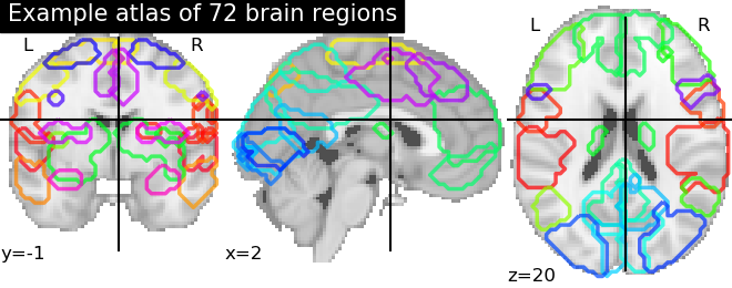
Basic atlas plotting

We use Nilearn plotting capabilities to plot and visualize our atlas in a convenient way

plotting.plot_prob_atlas(maps_img=os.path.join(home_directory, atlas_file_name),
                         title="Example atlas of 72 brain regions")

Out:

/home/dhaif/anaconda3/envs/conpagnon/lib/python3.7/site-packages/nilearn/plotting/displays.py:98: UserWarning: No contour levels were found within the data range.
  **kwargs)

<nilearn.plotting.displays.OrthoSlicer object at 0x7f3cb3d20278>

Atlas with no supplementary information

Sometimes, you won’t have at disposal the segmentation of the atlas in networks, or you won’t have a particular set of colors for the labels. In that case, you can simply import the atlas, and generate random colors:

# We can call fetch_atlas to retrieve useful information about the atlas
atlas_nodes, labels_regions, labels_colors, n_nodes = atlas.fetch_atlas(
    atlas_folder=home_directory,
    atlas_name=atlas_file_name,
    normalize_colors=False)

Now the label of a region is just the number of the region in the atlas, since we did not provide a label file:

# The labels of each region in now just a number
print(labels_regions)

Out:

[ 0  1  2  3  4  5  6  7  8  9 10 11 12 13 14 15 16 17 18 19 20 21 22 23
 24 25 26 27 28 29 30 31 32 33 34 35 36 37 38 39 40 41 42 43 44 45 46 47
 48 49 50 51 52 53 54 55 56 57 58 59 60 61 62 63 64 65 66 67 68 69 70 71]