Extracting brain signals

What you’ll learn: Extracting the signal for each regions in a brain atlas.

Author: Dhaif BEKHA

Retrieve the data

We will work on the dataset of the first tutorial. You can simply download it here, and go through all the necessary steps to organize your data. If you doesn’t want to go through all those steps, you can download the results, that is the dictionary containing all the necessary to the data files paths. We will also need a brain atlas. You can pick the one from the tutorial examples, or fetch your own.

Important

As usual ,we will work in the user home directory.

Modules import

from pathlib import Path
import os
from conpagnon.computing.compute_connectivity_matrices import time_series_extraction
from conpagnon.utils.folders_and_files_management import load_object, save_object
import numpy as np
import pandas as pd
import seaborn as sns
import matplotlib.pyplot as plt
from warnings import warn

Setting paths, and parameters

As usual, we set all the necessary path to the data, and we also load the data dictionary that you’ve just downloaded.

# Fetch the path of the home directory
home_directory = str(Path.home())

# The root fmri data directory containing all the fmri files directories
# This is the 'data' folder in you're home directory
root_fmri_data_directory = os.path.join(home_directory, 'data')

# Groups to include in the study: this is
# simply the name of the folder
group = ['group_1']

# Filename of the atlas file.
atlas_file_name = 'atlas.nii'
# Full path to the atlas file
atlas_path = os.path.join(home_directory, atlas_file_name)

# Repetition time in your resting state
# sequence
t_r = 2.4

# load the data dictionary, containing
# all the paths to the functional files for
# the groups in your study
groups_data_dictionary = load_object(
    full_path_to_object=os.path.join(home_directory, 'data_dictionary.pkl'))

# Full path to the text file containing the subjects identifiers
subjects_text_list = os.path.join(root_fmri_data_directory, 'text_data/subjects_list.txt')

# Create a cache directory for Nilearn
# when we will compute the times series
if 'nilearn_cache' not in os.listdir(home_directory):
    os.mkdir(os.path.join(home_directory, 'nilearn_cache'))

Compute the times series

Now we can call conpagnon.computing.compute_connectivity_matrices.time_series_extraction() function to compute in each brain region of the atlas, and for each subject the brain signals, commonly called times series.

# Compute the times series for each subject
times_series_dictionary = time_series_extraction(
    root_fmri_data_directory=root_fmri_data_directory,
    groupes=group,
    subjects_id_data_path=subjects_text_list,
    reference_atlas=atlas_path,
    group_data=groups_data_dictionary,
    repetition_time=t_r,
    nilearn_cache_directory=os.path.join(home_directory, 'nilearn_cache'))

The result is also a structured dictionary, following the same construction as the data dictionary. Let’s take a look, at the available fields for the subject 1 for example:

# Print the dictionary key for the first subject
print(times_series_dictionary['group_1']['subject_1'].keys())

Out:

dict_keys(['time_series', 'masked_array'])

The times_series field contain a numpy array, storing the brain signal for each regions. The field masked_array also contain a numpy array with boolean values of shape (number_of_brain_regions, number_of_brain_region). How to to possibly used the masked_array field will be discussed in the advanced examples section. Now, if we print the shape of shape of the times_series array we get:

print(times_series_dictionary['group_1']['subject_1']['time_series'].shape)

Out:

(180, 72)

The times_series array shape is (180, 72): 72 simply represent the number of region in the atlas we use, so yours may differ. 180, represent the number of time point in our functional image.

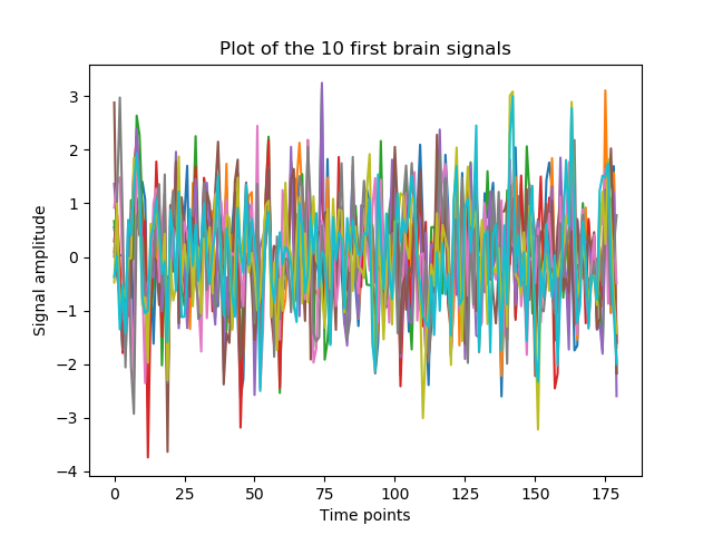
Plot the time series

We can plot the time series to visualize the brain signal we’ve just extracted, for the first subject. For obvious visualization purposes, we will plot the first 10 regions only

# number of region to plot
n_regions_to_plot = 10
# Times series of the first subject
subject_1_time_series = times_series_dictionary['group_1']['subject_1']['time_series']
# The time series time point:
time_points = np.arange(start=0, stop=subject_1_time_series.shape[0], step=1)
# Region number
region_number = np.arange(start=0, stop=subject_1_time_series.shape[1], step=1)
# Build a panda dataframe: each column contain the associated brain signal in that
# region number
times_series_dataframe = pd.DataFrame(subject_1_time_series, time_points, region_number).T
# plot the time series
for i in range(n_regions_to_plot):
    ax = sns.lineplot(x=time_points, y=times_series_dataframe.loc[i])
    ax.set_xlabel('Time points')
    ax.set_ylabel('Signal amplitude')
    ax.set_title('Plot of the {} first brain signals'.format(n_regions_to_plot))
plt.show()

Out:

/media/dhaif/Samsung_T5/Work/Programs/ConPagnon/examples/02_Functional_Connectivity/plot_times_series_extraction.py:151: UserWarning: Matplotlib is currently using agg, which is a non-GUI backend, so cannot show the figure.
  plt.show()

Note

As you can see, those brain signals seem to be very similar ! The times series are usually not the primary object we will manipulate in the statistical analysis. Indeed, the traditional next step should be the computation of the connectivity matrices explain in the next section.

Save the times series dictionary

For convenience, you can save the times series dictionary in you’re home directory:

# Save the times series dictionary
save_object(object_to_save=times_series_dictionary,
            saving_directory=home_directory,
            filename='time_series_dictionary.pkl')