Two groups classification

What you’ll learn: Perform a simple classification between two distinct group of subjects, and evaluate the accuracy for different connectivity metric.

Author: Dhaif BEKHA

Retrieve the example dataset

In this example, we will work directly on a pre-computed dictionary, that contain two set of connectivity matrices, from two different groups. The first group, called controls is a set of connectivity matrices from healthy seven years old children, and the second group called patients, is a set of connectivity matrices from seven years old children who have suffered a stroke. You can download the dictionary use in this example here.

Module import

from conpagnon.utils.folders_and_files_management import load_object, save_object
import numpy as np
from nilearn.connectome import sym_matrix_to_vec
from sklearn.model_selection import cross_val_score, StratifiedShuffleSplit
from sklearn.svm import LinearSVC
import matplotlib.pyplot as plt
import seaborn as sns
from matplotlib.backends.backend_pdf import PdfPages
import os
from pathlib import Path

Load data, and set Path

We will load the pre-computed dictionary containing the connectivity matrices for each subjects, for different metrics. We already used this exact same dictionary in the t-test example.

# Fetch the path of the home directory
home_directory = str(Path.home())

# Load the dictionary containing the connectivity matrices
subjects_connectivity_matrices = load_object(
    full_path_to_object=os.path.join(home_directory, 'raw_subjects_connectivity_matrices.pkl'))

# Fetch tne group name, for this classification
# task, the group name are the class name too.
groups = list(subjects_connectivity_matrices.keys())

Classification between the two group

We will compute a classification task for each connectivity at disposal, between the two group. In this example, we will use a classical support vector machine (SVM) algorithm with a linear kernel. We will leave the hyperparameters by default. First we create the labels for each class, that is simply create a 1D vector with binary labels. We naturally cross validate our results with a Stratified Shuffle and Split strategy. The evaluation metric of classification scores, will be the accuracy. The features are simply the connectivity coefficient , and we take the lower triangle only, because of the symmetry of the connectivity matrices. We have to vectorize each matrices in order to produce a data array of shape (n_subjects, n_features).

# Labels vectors: 0 for the first class, 1 for the second. Those
# 1, and 0 are the label for each subjects.
class_labels = np.hstack((np.zeros(len(subjects_connectivity_matrices[groups[0]].keys())),
                          np.ones(len(subjects_connectivity_matrices[groups[1]].keys()))))

# total number of subject
n_subjects = len(class_labels)

# Stratified Shuffle and Split cross validation:
# we initialize the cross validation object
# and set the split to 10000.
cv = StratifiedShuffleSplit(n_splits=10000,
                            random_state=0)

# Instance initialization of SVM classifier with a linear kernel
svc = LinearSVC()

# Compare the classification accuracy across multiple metric
metrics = ['tangent', 'correlation', 'partial correlation']
mean_scores = []

# To decrease the computation time you
# can distribute the computation on
# multiple core, here, 4.
n_jobs = 4

# Final mean accuracy scores will be stored in a dictionary
mean_score_dict = {}
for metric in metrics:
    # We take the lower triangle of each matrices, and vectorize it to
    # produce a classical machine learning data array of shape (n_subjects, n_features)
    features = sym_matrix_to_vec(np.array([subjects_connectivity_matrices[group][subject][metric]
                                           for group in groups
                                           for subject in subjects_connectivity_matrices[group].keys()],
                                          ), discard_diagonal=True)
    print('Evaluate classification performance on {} with '
          '{} observations and {} features...'.format(metric, n_subjects, features.shape[1]))
    # We call cross_val_score, a convenient scikit-learn
    # wrapper that will perform the classification task
    # with the desired cross-validation scheme.
    cv_scores = cross_val_score(estimator=svc, X=features,
                                y=class_labels, cv=cv,
                                scoring='accuracy', n_jobs=n_jobs)
    # We compute the mean cross-validation score
    # over all the splits
    mean_scores.append(cv_scores.mean())
    # We store the mean accuracy score
    # in a dictionary.
    mean_score_dict[metric] = cv_scores.mean()
    print('Done for {}'.format(metric))

Out:

Evaluate classification performance on tangent with 53 observations and 2556 features...
Done for tangent
Evaluate classification performance on correlation with 53 observations and 2556 features...
Done for correlation
Evaluate classification performance on partial correlation with 53 observations and 2556 features...
Done for partial correlation

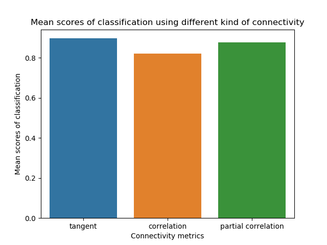
Barplot of the accuracy

We can plot the accuracy for each metric in a barplot. We simply use the dictionary in which we stored the accuracy score for each metric.

plt.figure()
sns.barplot(x=list(mean_score_dict.keys()), y=list(mean_score_dict.values()))
plt.xlabel('Connectivity metrics')
plt.ylabel('Mean scores of classification')
plt.title('Mean scores of classification using different kind of connectivity')
plt.show()

Out:

/media/dhaif/Samsung_T5/Work/Programs/ConPagnon/examples/03_Basic_Statistical_Analyses/plot_two_groups_classification.py:138: UserWarning: Matplotlib is currently using agg, which is a non-GUI backend, so cannot show the figure.
  plt.show()

Important

As you can see, the accuracy vary between connectivity metric. The tangent metric present the best accuracy scores here. So if classification is your main objective, you should choose very carefully the metric. Different machine learning algorithm will perform differently, I encourage you to test multiple algorithm on your data.